APPENDIX I
Polar Variations

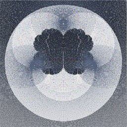
Polar Variations use Julia Unit Circle variations with polar coodinates and trigonometric functions.
See Appendix B for a different aspect of this configuration type and further discussion.

Polar Example

Polar Example with Pseudocode

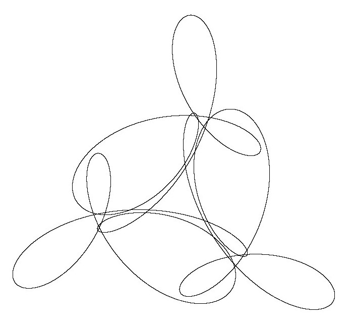
for (int i = 0; i ≤ 1000000; i++) {
	x = 0.0;
	y = 0.0;
	for (k = 3; k ≤ 6; k++)	{
		θ = 2.0k * i * 0.0001;
		xnew = y + 2.0 * cos(θ);
		ynew = x + 2.0 * sin(θ);
		x = xnew;
		y = ynew;
	}
	PlotPoint(x * scale, y * scale, color);
}

Polar	Map	Build (f(θ,x,y), g(θ,x,y))	kmin, kmax	Plot
Example	θ	(y + 2.0 * cos(θ), x + 2.0 * sin(θ))	3, 6	Point
Polar #1	θ	(cos(θ + k) + x, sin(θ + k) + y)	9, 13	Point
Polar #2	θ	(cos(θ) + x * 0.5, sin(θ) - y * 0.5)	6, 9	Point
Polar #3	θ	(cos(θ) + y * 0.75, sin(θ) - x * 0.5)	6, 9	Point
Polar #4	θ	(cos(θ + k) + x * y, sin(θ + k) + x * y)	9, 13	Point
Polar #5	θ	(y + cos(y + θ), x + sin(x + θ))	3, 6	Point
Polar #6	θ	(y + cos(θ) - 0.25 * x, x + sin(θ) + 0.25 * y)	3, 7	Point
Polar #7	θ	(cos(θ * k) + x * 0.5, sin(θ * k) - y * 0.5)	9, 10	Point
Polar #8	θ	(cos(θ * k) + x * 0.5, sin(θ * k) - y * 0.5)	2, 4	Point
Polar #9	θ	(cos(θ * k) - x * 0.5, sin(θ * k) - x*y * 0.5)	2, 4	Point
Polar #10	θ	(y * cos(θ * k) - x * 0.5, sin(θ * k) - y * 0.5)	2, 4	Point
Polar #11	θ	(cos(θ * k) - x * 0.5, (cos(θ * k) - x * 0.5) * sin(θ * k) - y * 0.5)	2, 3	Point
Polar #12	θ	(x * y + cos(θ * k) - x * 0.5, sin(θ * k) - y * 0.5)	2, 4	Point

Polar #1

Polar #2

Polar #3

Polar #4

Polar #5

Polar #6

Polar #7

Polar #8

Polar #9

Polar #10

Polar #11

Polar #12